Complexity control
Version: 1.0.0
Pattern language family: BN
Modeling phase:
2. The conceptualization phase of a system of interest
3. The technical implementation
Modeling step:
    6. Choice of estimation performance criteria and technique
    7. Identification of model structure and parameters' values
Problem:
BNs can become computationally intractable with the increase of their complexity. A network complexity can be represented by the maximum size of its CPTs. The size of a node’s CPT grows exponentially with the increase of the number of its parents and their respective states. The network complexity can then be represented as:
\[max(CPT(d))= d^s \prod_{i=1}^{n} P_{i}^{s}\]where: $CPT(d)$ is the size of the CPT for a node $d$, $d^s$ is the number of states for a discrete node $d$, and $P_{i}^{s}$ is the number of states of the ith parent of node $d$.
Solution:
In order to decrease complexity we need to decrease the maximum CPT size. This can be achieved by reducing the number of parents for the nodes which CPT size surpasses a preset threshold, e.g.$2^{16}$. This is done through:
-
Application of the Local dependence confirmation pattern which entails excluding the parents that are highly correlated for the node under consideration.
-
Applying node divorcing, i.e. grouping the parents that are logically related and adding a new latent node that acts as a child for each parent group. These latent nodes can then act as parents for the node with the complex CPT.
By applying this solution the size of the CPT for complex child node will be reduced as the number of parents will be decreased, hence the complexity of the network will be reduced. A side effect for this solution is that the previously complex node, e.g. node $y`$ in Fig.1, will be less sensitive to changes in the originally parent nodes, e.g. nodes $X_1$ to $X_5$.
Structure: The solution proposed by this pattern have the following structure in a BN:
In Fig.1 below, N1 is the complex node before divorcing and N2 is the less complex network after introducing two latent variables, $A$ to group ${X_1, X_2, X_3}$ and $B$ to group ${X_4, X_5}$. $y’$ has a smaller CPT than $y$.
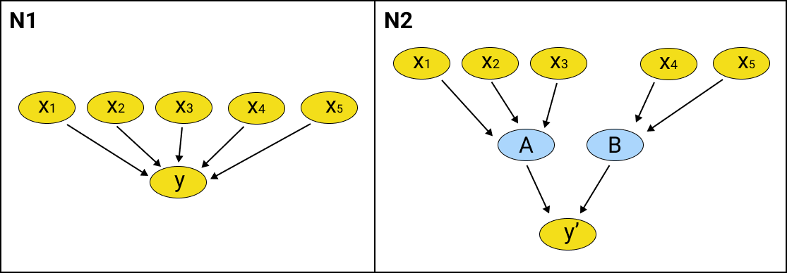
Fig.1 The model structure before and after applying the node divorcing solution.
Constraints:
This solution works under the following conditions:
-
There should be a logical connection between the grouped parents, otherwise they cannot be grouped.
-
As "node divorcing" adds intermediate nodes between parent nodes and child nodes, if the parent node is an intervention node, divorcing can "dilute" the impact of the intervention, i.e. reduce the sensitivity of the child to changes in the distribution of the parent.
Related patterns:
Design choice and model quality:
- 2.F
- 2.R
Resources:
-
Marcot, B. G. (2012). Metrics for evaluating performance and uncertainty of Bayesian network models. Ecological modelling, 230, 50-62.
-
Marcot, B. G. (2017). Common quandaries and their practical solutions in Bayesian network modeling. Ecological Modelling, 358, 1-9.
-
McCann, R. K., Marcot, B. G., & Ellis, R. (2006). Bayesian belief networks: applications in ecology and natural resource management. Canadian Journal of Forest Research, 36(12), 3053-3062.
-
von Waldow, U., & Röhrbein, F. (2015). Structure Learning in Bayesian Networks with Parent Divorcing. In EAPCogSci.
-
Cain, J. (2001). Planning improvements in natural resources management. Centre for Ecology and Hydrology, Wallingford, UK, 124, 1-123.