Making things happen
Version: 1.0.0
Pattern language family: BN
Modeling phase:
3. The technical implementation
5. Communication of model findings
Modeling step:
7. Identification of model structure and parameters' values
9. Quantification of uncertainty
Problem:
One of the main applications of BNs is using them to explore the potential behavior of a system after manipulating some variables in that system. In causal BNs, such manipulations are known as Interventions. This pattern defines the different types of interventions and how they can be introduced to BNs in an effective manner.
Solution:
An intervention is an exogenous influence on some system that acts on a certain component of that system. For the causal BN $(G)$ representing that system, an intervention on a variable $v \in G$ transforms $G$ into the extended BN $(G’)$ by adding the node $I_v \rightarrow v$ to $G$, where:
-
$I_v$ is introduced to intentionally change $v$ so that a target distribution $P^(v)$ over the states of $v$ is achieved. However, $I_v$ does not restrict the influence of other parents of $v$, which means that the target $P^(v)$ might not be actually achieved (see below the special case “perfect intervention”).
-
$I_v$ is a parent of $v$.
-
$I_v$ is a binary variable indicating whether the intervention is activated or not.
A perfect intervention on a variable will cut off all influence of the parents of that variable causing the variable to adopt a unique state. An intervention, however, will have an influence on the variable’s state, but not to the extreme of cutting off all its parents’ effect. Although a perfect intervention is simpler in application and calculation, it is unable to represent many realistic scenarios, see below Figure 1 for details of the impacts of both. It is worth noting that describing an intervention as perfect does not imply it is better or more effective. Actually, it is recommended that BNs’ users utilize interventions and avoid perfect interventions as the latter over-simplifies the model.

Fig.1 The impact of the perfect intervention ($R_Y$) against the intervention ($I_Y$) on the network. When $R_Y$ is introduced to the network as a perfect intervention on the variable $Y$, it cuts off the influence of its parent $X$ and sets the probability of the intervened upon state to $1$. While when $I_Y$ is introduced to $Y$, it does not cut off the influence of $X$, however it affects the probability distribution of the states of $Y$.
In order to properly introduce interventions to the model, BN users are advised against changing the states of variables through evidence updating. BN users should also refrain from introducing interventions as new observations to the variables as this will lead to the model producing inaccurate results. Interventions, however, are recommended to be modeled by augmenting the graph $G$ with additional intervention nodes for every intervened upon variable. The details of building intervention-augmented BN is as follows:
-
Define the set of variables to be targeted by interventions $V= {v_1,..,v_n}$.
-
For every variable $v_i \in V$ define the intervention(s) $I_{v_i}$ targeting $v_i$. Such definition indicate the probability distribution implied by $I_{v_i}$ over the states of the variable $S_{v_i}$.
-
Create $G’$ by making a copy of $G$ and substituting the node $v_i$ with a new Noisy-MAX copy of $v_i$ (for details about the Noisy-MAX nodes see [4]).
-
In $G’$ add $I_{v_i}$ as a parent for $v_i$.
-
Modify the CPT of $v_i$ to show the desired effect of $I_{v_i}$, e.g. $p(S_{v_i} = {s_1, s_2} \vert I_{v_i}=present) = {1, 0}$ which means that the probabilities of the $v_i$ states $s_1$ and $s_2$ given that the intervention $I_{v_i}$ is present are $1$ and $0$ respectively. Such distribution implies that we are forcing $s_1$. The probabilities of the other parents of $v_i$ will be similar to their original probabilities in $G$.
-
Changing the states of the intervention variable $I_{v_i}$ will then reflect the effect of intervention on the variables in the network.
In BN models, interventions can be used for several purposes. The most common are:
-
To use BNs as decision support systems, by introducing different policies as interventions and study the effect of each policy on the system outcomes.
-
Interventions can be used to facilitate scenario modeling by defining scenarios as sets of interventions that act on certain variables in the BN.
-
Interventions can be used to verify the causal relationship between multiple variables included in the network as well as verifying the faithfulness of the BN to the system it aims to model (see the pattern “BN causality” for more details).
Structure: The structure for this solution can be shown through the following example:
Consider the model in Figure 2 that aims at representing the impacts of innovation, economic efficiency, and equity on the social and environmental components of sustainability. Assume that there is a new policy to be introduced that will reduce some environment related restrictions on industry, and as a consequence will have negative impacts on the environmental component of sustainability. In order to model this intervention, we follow the steps mentioned in the solution section.
-
First define the variables that will be targeted by the intervention, which is Environmental in this case.
-
Then we define the intervention variable $I_env$ as a binary variable that has the states ${present, absent}$. After that we define the probability distribution implied by $I_{env}$ on the states of environmental. If we are certain that the intervention will cause environmental to be in the low state, then the probability distribution should be $p(environmental=low \vert I_{env}=present)=1$. However, we assume that we are uncertain about the impacts of $I_{env}$, hence, $p(environmental=low \vert I_{env}=present)=0.7$.
-
We create $G’$, shown in Figure 2, (b), by copying the network in Figure 2, (a) and substituting Environmental with the a node of Noisy-MAX type.
-
Add the intervention node $I_{env}$ to $G’$ as a parent of Environmental_copy.
-
Modify the CPT of Environmental_copy to reflect the expected impact of the intervention. As shown in Figure 3, when the $I_{env}$ is present, there is a $0.7$ probability that Environmental_copy will be in the Low state. The distribution of the Econ-Eff_copy is similar to its counterpart Economic-Efficiency. As it appears in Figure 2 the probabilities in $G$ and $G’$ are similar at the absence of the intervention.
-
Changing the state of $I_{env}$ to present will cause a change of the probabilities of Environmental_copy and its descendent Sustainability_copy. The intervention is expected to increase the probability of Environmental_copy to be in the low state from $16\%$ to $75\%$ and increase the probability of Sustainability_copy to be in the Negative state from $11\%$ to $21\%$.
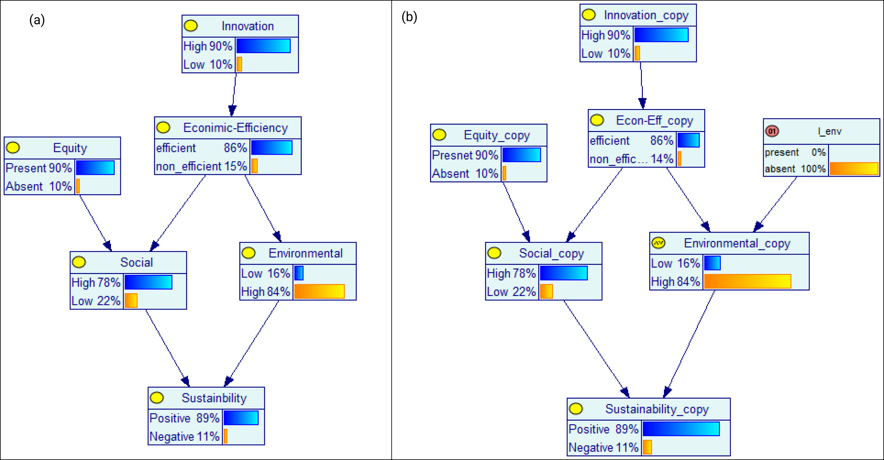
Fig.2 An example BN model. (a) shows the original BN, and (b) shows the Intervention-augmented copy.
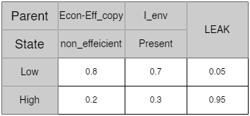
Fig.3 The CPT of the Noisy-MAX node Environmental_copy.
Constraints:
The following assumptions are considered when presenting interventions to BNs:
-
Interventions themselves are uncaused, this means that the nodes representing interventions in the network are parentless, i.e. root nodes.
-
Multiple interventions are uncorrelated.
-
An intervention node in the model acts upon only one variable in the model. From an OOP point of view, this is related to the concept of Single-Responsibility principle as the variable intervened upon will only change based on the single intervention related to it.
-
Interventions should not be confused with observations (check the pattern BNs Causality for a comparison between the two concepts). Interventions allow us to perform causal reasoning, while observations are only useful for observational, or probabilistic, reasoning.
-
The intervention node and the intervened upon node need to be discrete variables.
Related patterns:
Design choice and model quality:
- 1.U
- 2.U
- 3.R
Resources:
-
Korb, K. B., Hope, L. R., Nicholson, A. E., & Axnick, K. (2004, August). Varieties of causal intervention. In Pacific Rim international conference on artificial intelligence (pp. 322-331). Springer, Berlin, Heidelberg.
-
Korb, K. B., & Nicholson, A. E. (2008). The causal interpretation of Bayesian networks. In Innovations in Bayesian Networks (pp. 83-116). Springer, Berlin, Heidelberg.
-
Zagorecki, A. T. (2010). Local probability distributions in Bayesian networks: Knowledge elicitation and inference. University of Pittsburgh.
-
Zagorecki, A., & Druzdzel, M. J. (2012). Knowledge engineering for Bayesian networks: How common are noisy-MAX distributions in practice?. IEEE Transactions on Systems, Man, and Cybernetics: Systems, 43(1), 186-195.